The Cookies model

Overview

This model implements the so-called ‘cookies problem’ or ‘cookies in the oven problem’ (see for reference [Bäck et al.,2011], [Ballani et al.,2015], [Kressner et al., 2011]), i.e., a simplified thermal equation in which the conductivity coefficient is uncertain in 8 circular subdomains (‘the cookies’), whereas it is known (and constant) in the remaining of the domain (‘the oven’). The equation can be either stationary (elliptic PDE) or time-dependent (parabolic PDE). The spatial approximation is constructed using the legacy version of FEniCs via the Python interface, using quadrilateral meshes (FEM degree configurable by the user); the time-advancing scheme is adaptive with local error control, specifically an implementation of the TR-AB2 scheme, see, e.g., [Iserles, 2008]. See below for full description.

Authors

• Benjamin Kent

• Massimiliano Martinelli

• Lorenzo Tamellini

Run

docker run -p 4242:4242 -it linusseelinger/cookies-problem:latest

Properties

The Docker container serves three models, two for the elliptic version of the PDE and one for the parabolic one.

Model	Description
forward	Forward evaluation of the elliptic version of the cookies model, all config options can be modified by the user (see below)
forwardparabolic	Forward evaluation of the parabolic version of the cookies model, all config options can be modified by the user (see below)
benchmark	Sets the config options for the forward UQ benchmark (see benchmark page)

forward

Mapping	Dimensions	Description
input	[8]	These values modify the conductivity coefficient in the 8 cookies, each of them must be greater than -1 (software does not check that input values are valid)
output	[1]	The integral of the solution over the central subdomain \(F\) (see below for details)

Feature	Supported
Evaluate	True
Gradient	False
ApplyJacobian	False
ApplyHessian	False

Config	Type	Default	Description
N	integer	400	The number of cells in each dimension (i.e. a mesh of \(N^2\) elements).
Fidelity	integer	4	If provided, the mesh will be generated with N = 100 x Fidelity. The ‘fidelity’ config key takes precedent over ‘N’ if both defined.
BasisDegree	Integer	1	The degree of the piecewise polynomial FE approximation
advection	Integer	0	A flag to add an an advection field to the problem. If set to 1 an advection term with advection field (see below) is added to the PDE problem.
quad_degree	Integer	8	The quadrature degree used to evaluate integrals in the matrix assembly.
diffzero	Float	1.0	Defines the background diffusion field \(a_0\) (see below)
directsolver	Integer	1	Uses a direct LU solve for linear system. Set to 0 to use GM-RES.
pc	String	‘none’	Preconditioning for the GM-RES solver, can be either ‘ILU’ or ‘JACOBI’
tol	Float	1e-4	Relative tolerance for the GM-RES solver.

forwardparabolic

Mapping	Dimensions	Description
input	[8]	These values modify the conductivity coefficient in the 8 cookies, each of them must be greater than -1 (software does not check that input values are valid)
output	[1]	The integral of the solution over the central subdomain \(F\) (see below for details)

Feature	Supported
Evaluate	True
Gradient	False
ApplyJacobian	False
ApplyHessian	False

Config	Type	Default	Description
N	integer	400	The number of cells in each dimension (i.e. a mesh of \(N^2\) elements).
Fidelity	integer	4	If provided, the mesh will be generated with N = 100 x Fidelity. The ‘fidelity’ config key takes precedent over ‘N’ if both defined.
BasisDegree	Integer	1	The degree of the piecewise polynomial FE approximation
advection	Integer	0	A flag to add an an advection field to the problem. If set to 1 an advection term with advection field (see below) is added to the PDE problem.
quad_degree	Integer	8	The quadrature degree used to evaluate integrals in the matrix assembly.
diffzero	Float	1.0	Defines the background diffusion field \(a_0\) (see below)
letol	Float	1e-4	Local timestepping error tolerance for a simple implementation of TR-AB2 timestepping.
T	Float	10.0	Final time for timestepping approximation. The QoI is evaluated and returned for time T.

Mount directories

Mount directory	Purpose
None

Source code

Model sources here.

Description

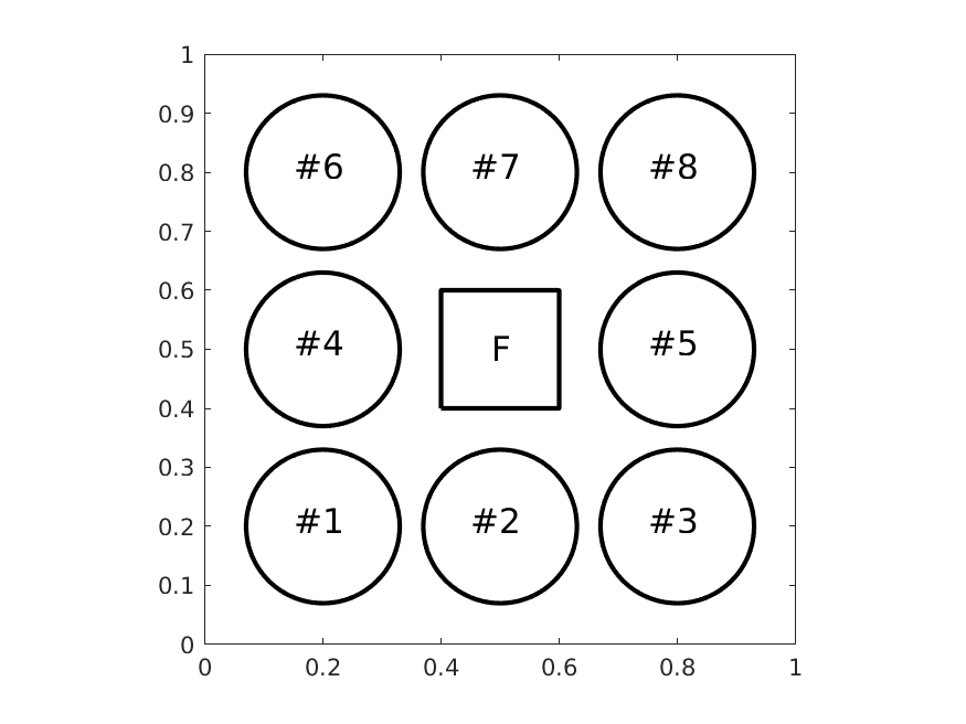
In its elliptic variant, the model implements the version of the cookies problem in [Bäck et al.,2011], see also e.g. [Ballani et al.,2015], [Kressner et al., 2011] for slightly different versions. With reference to the computational domain \(D=[0,1]^2\) in the figure above, the cookies model consists in the thermal diffusion problem below, where \(\mathbf{y}\) are the uncertain parameters discussed in the following and \(\mathrm{x}\) are physical coordinates.

\[-\mathrm{div}\Big[ a(\mathbf{x},\mathbf{y}) \nabla u(\mathbf{x},\mathbf{y}) \Big] = f(\mathrm{x}), \quad \mathbf{x}\in D\]

with homogeneous Dirichlet boundary conditions and forcing term defined as

\[\begin{split}f(\mathrm{x}) = \begin{cases} 100 &\text{if } \, \mathrm{x} \in F \\ 0 &\text{otherwise} \end{cases}\end{split}\]

where \(F\) is the square \([0.4, 0.6]^2\). The 8 subdomains with uncertain diffusion coefficient (the cookies) are circles with radius \(0.13\) and the following center coordinates:

cookie	1	2	3	4	5	6	7	8
x	0.2	0.5	0.8	0.2	0.8	0.2	0.5	0.8
y	0.2	0.2	0.2	0.5	0.5	0.8	0.8	0.8

The uncertain diffusion coefficient is defined as

\[a = a_0 + \sum_{n=1}^8 y_n \chi_n(\mathrm{x})\]

where \(a_0=1\) by default (can be changed by the user), \(y_n > -1\) and

\[\begin{split}\chi_n(\mathrm{x}) = \begin{cases} 1 &\text{inside the n-th cookie} \\ 0 &\text{otherwise} \end{cases}\end{split}\]

The output of the simulation is the integral of the solution over \(F\), i.e. \(\Psi = \int_F u(\mathrm{x}) d \mathrm{x}\)

An advection term can be added to the equation, by suitably setting the config options. In this case, the equation becomes

\[-\mathrm{div}\Big[ a(\mathbf{x},\mathbf{y}) \nabla u(\mathbf{x},\mathbf{y}) \Big] + \mathbf{w}(\mathbf{x}) \cdot \nabla u(\mathbf{x},\mathbf{y}) = f(\mathrm{x}), \quad \mathbf{x}\in D\]

with \(\mathbf{w}(\mathbf{x})= [4(x_2-0.5)(1-4(x_1-0.5)^2), \,\, -4(x_1-0.5)*(1-4(x_2-0.5)^2)].\)

The PDE is solved by a classical Finite Eement Method (using the legacy version of FEniCs via the Python interface), with standard Lagrangian polynomial bases of degree \(p\) ove quadrilateral meshes (FEM degree configurable by the user). The meshes contain \(100\times K\) elements per direction. The corresponding linear system can be solvers either directly (LU solver) or iteratively by GMRES method, with three choices of preconditioning (none, ILU, Jacobi), up to the users. The relative tolerance of the iterative method can also be set by the user.

A parabolic (time-dependent) variant of the same problem is provided, that can be selected by using the forwardparabolic model introduced above. In this case, the equation becomes

\[\displaystyle \frac{\partial u(\mathbf{x},t,\mathbf{y})}{\partial t} -\mathrm{div}\Big[ a(\mathbf{x},\mathbf{y}) \nabla u(\mathbf{x},\mathbf{y}) \Big] + \mathbf{w}(\mathbf{x}) \cdot \nabla u(\mathbf{x},t,\mathbf{y}) = f(\mathrm{x}), \quad \mathbf{x}\in D, t \in (0,T]\]

with \(T\) specified by the user and initial condition \(u=0\). Like in the elliptic case, the advection term is null by default. All config options of the elliptic variant can be used here. Concerning time-stepping, the time-advancing scheme is adaptive with local error control, specifically an implementation of the TR-AB2 scheme, see, e.g., [Iserles, 2008].