Deconvolution1D

Overview

This benchmark is based on a 1D Deconvolution test problem from the library CUQIpy. It defines a posterior distribution for a 1D deconvolution problem, with a Gaussian likelihood and four different choices of prior distributions with configurable parameters.

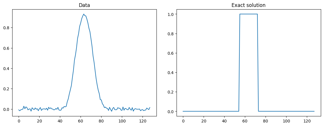
Plot of data and exact solution

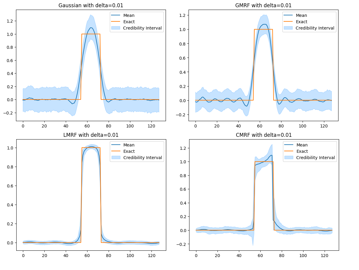
Credibility interval plots of posterior samples using different priors

Authors

• Nicolai A. B. Riis

• Jakob S. Jørgensen

• Amal M. Alghamdi

Run

docker run -it -p 4243:4243 linusseelinger/benchmark-deconvolution-1d:latest

Properties

Model	Description
Deconvolution1D_Gaussian	Posterior distribution with Gaussian prior
Deconvolution1D_GMRF	Posterior distribution with Gaussian Markov Random Field prior
Deconvolution1D_LMRF	Posterior distribution with Laplacian Markov Random Field prior
Deconvolution1D_CMRF	Posterior distribution with Cauchy Markov Random Field prior
Deconvolution1D_ExactSolution	Exact solution to the deconvolution problem

Deconvolution1D_Gaussian

Mapping	Dimensions	Description
input	[128]	Signal \(\mathbf{x}\)
output	[1]	Log PDF \(\pi(\mathbf{b}\mid\mathbf{x})\) of posterior with Gaussian prior

Feature	Supported
Evaluate	True
Gradient	True
ApplyJacobian	False
ApplyHessian	False

Config	Type	Default	Description
delta	double	0.01	The prior parameter \(\delta\) (see below).

Deconvolution1D_GMRF

Mapping	Dimensions	Description
input	[128]	Signal \(\mathbf{x}\)
output	[1]	Log PDF \(\pi(\mathbf{b}\mid\mathbf{x})\) of posterior with Gaussian Markov Random Field prior

Feature	Supported
Evaluate	True
Gradient	True
ApplyJacobian	False
ApplyHessian	False

Config	Type	Default	Description
delta	double	0.01	The prior parameter \(\delta\) (see below).

Deconvolution1D_LMRF

Mapping	Dimensions	Description
input	[128]	Signal \(\mathbf{x}\)
output	[1]	Log PDF \(\pi(\mathbf{b}\mid\mathbf{x})\) of posterior Laplacian Markov Random Field prior

Feature	Supported
Evaluate	True
Gradient	False
ApplyJacobian	False
ApplyHessian	False

Config	Type	Default	Description
delta	double	0.01	The prior parameter \(\delta\) (see below).

Deconvolution1D_CMRF

Mapping	Dimensions	Description
input	[128]	Signal \(\mathbf{x}\)
output	[1]	Log PDF \(\pi(\mathbf{b}\mid\mathbf{x})\) of posterior with Cauchy Markov Random Field prior

Feature	Supported
Evaluate	True
Gradient	True
ApplyJacobian	False
ApplyHessian	False

Config	Type	Default	Description
delta	double	0.01	The prior parameter \(\delta\) (see below).

Deconvolution1D_ExactSolution

Mapping	Dimensions	Description
input	[0]	No input to be provided.
output	[128]	Returns the exact solution \(\mathbf{x}\) for the deconvolution problem.

Feature	Supported
Evaluate	True
Gradient	False
ApplyJacobian	False
ApplyHessian	False

Config	Type	Default	Description
None

Mount directories

Mount directory	Purpose
None

Source code

Sources here.

Description

The 1D periodic deconvolution problem is defined by the inverse problem

\[ \mathbf{b} = \mathbf{A}\mathbf{x} + \mathbf{e}, \]

where \(\mathbf{b}\) is an \(m\)-dimensional random vector representing the observed data, \(\mathbf{A}\) is an \(m\times n\) matrix representing the convolution operator, \(\mathbf{x}\) is an \(n\)-dimensional random vector representing the unknown signal, and \(\mathbf{e}\) is an \(m\)-dimensional random vector representing the noise.

This benchmark defines a posterior distribution over \(\mathbf{x}\) given \(\mathbf{b}\) as

\[ \pi(\mathbf{x}\mid \mathbf{b}) \propto \pi(\mathbf{b}\mid \mathbf{x})\pi(\mathbf{x}), \]

where \(\pi(\mathbf{b}|\mathbf{x})\) is a likelihood function and \(\pi(\mathbf{x})\) is a prior distribution.

The noise is assumed to be Gaussian with a known noise level, and so the likelihood is defined via

\[ \mathbf{b} \mid \mathbf{x} \sim \mathcal{N}(\mathbf{A}\mathbf{x}, \sigma^2\mathbf{I}_m), \]

where \(\mathbf{I}_m\) is the \(m\times m\) identity matrix and \(\sigma=0.01\) defines the noise level.

The prior can be configured by choosing of the following assumptions about \(\mathbf{x}\):

• Gaussian: Gaussian (Normal) distribution: \(x_i \sim \mathcal{N}(0, \delta)\).

• GMRF Gaussian Markov Random Field: \(x_i-x_{i-1} \sim \mathcal{N}(0, \delta)\).

• CMRF Cauchy Markov Random Field: \(x_i-x_{i-1} \sim \mathcal{C}(0, \delta)\).

• LMRF Laplace Markov Random Field: \(x_i-x_{i-1} \sim \mathcal{L}(0, \delta)\).

where \(\mathcal{C}\) is the Cauchy distribution and \(\mathcal{L}\) is the Laplace distribution. The parameter \(\delta\) is the prior parameter and is configurable (see above).

The choice of prior is specified by providing the name to the HTTP model. In this case Deconvolution1D_Gaussian, Deconvolution1D_GMRF, Deconvolution1D_CMRF, and Deconvolution1D_LMRF, respectively. See um-bridge Clients for more details.

In addition to the HTTP models for the posterior, there is also an HTTP model for the exact solution to the problem. This model is called Deconvolution1D_ExactSolution and returns exact phantom used to generate the synthetic data when called.

In CUQIpy the benchmark is defined and sampled as follows:

import numpy as np
import cuqi

# Parameters
delta = 0.01
prior = "LMRF"

# Load data, define problem and sample posterior
TP = cuqi.testproblem.Deconvolution1D(
    dim=128,
    PSF="gauss",
    PSF_param=5,
    phantom="square",
    noise_std=0.01,
    noise_type="gaussian"
)
if prior == "Gaussian":
    TP.prior = cuqi.distribution.Gaussian(np.zeros(128), delta)
elif prior == "GMRF":
    TP.prior = cuqi.distribution.GMRF(np.zeros(128), 1/delta)
elif prior == "CMRF":
    TP.prior = cuqi.distribution.CMRF(np.zeros(128), delta)
elif prior == "LMRF":
    TP.prior = cuqi.distribution.LMRF(np.zeros(128), delta)
TP.sample_posterior(2000).plot_ci(exact=TP.exactSolution)