Computed Tomography using CUQIpy¶

Overview¶

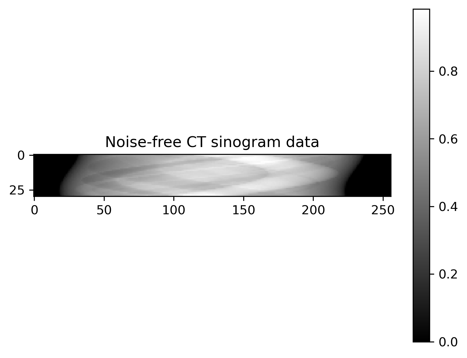
This benchmark focuses on image reconstruction in X-ray computed tomography (CT). In CT, X-ray are passed through an object of interest and projection images are recorded at all orientations. Materials of different density absorb X-rays by different amounts quantified by the linear attenuation coefficients. A linear forward model describes how the 2D linear attenuation image of an object results in a measured set of projections, typically known as a sinogram. The benchmark uses the library CUQIpy to specify the linear forward model, based on a matrix constructed with the library AIR Tools II. It defines a posterior distribution for a 2D X-ray CT image reconstruction problem problem, with a Gaussian noise distribution ie likelihood and four different choices of 2D prior distributions with configurable parameters.

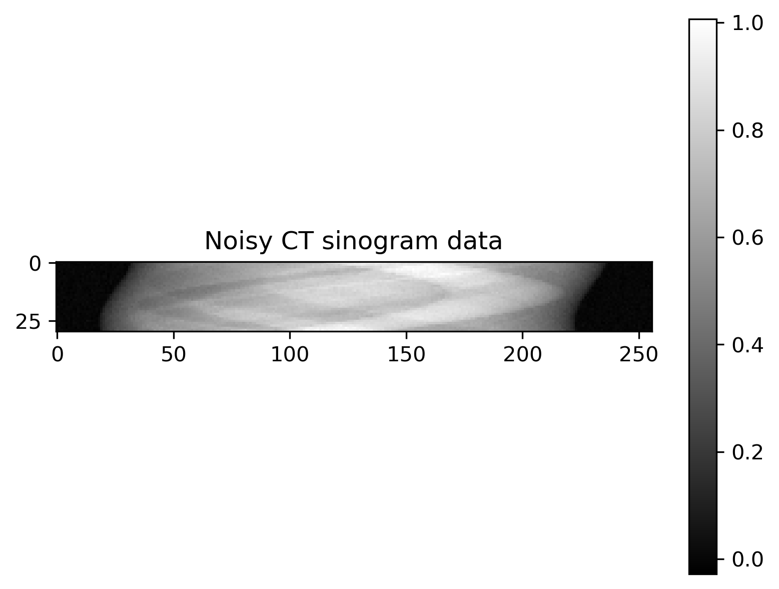
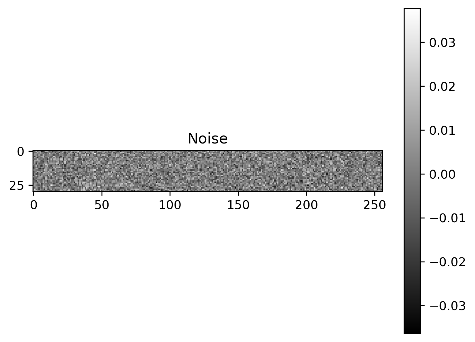
Plot of exact solution, noise-free data, noisy data and noise:

True image	Noise-free data

Noisy data	Noise

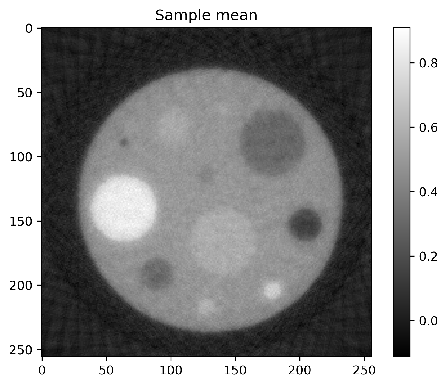
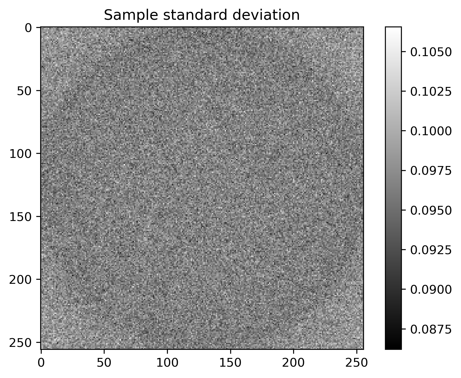
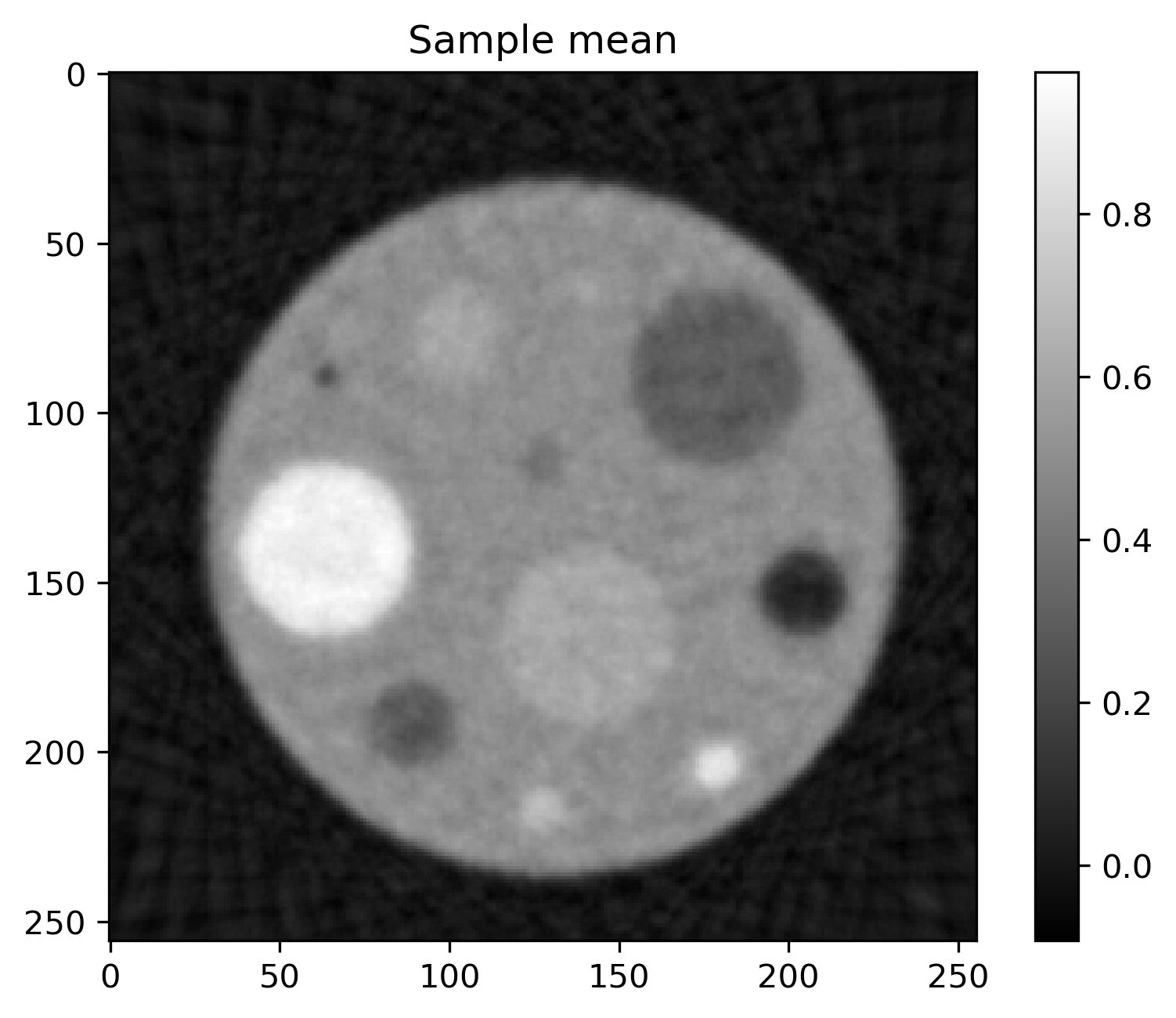
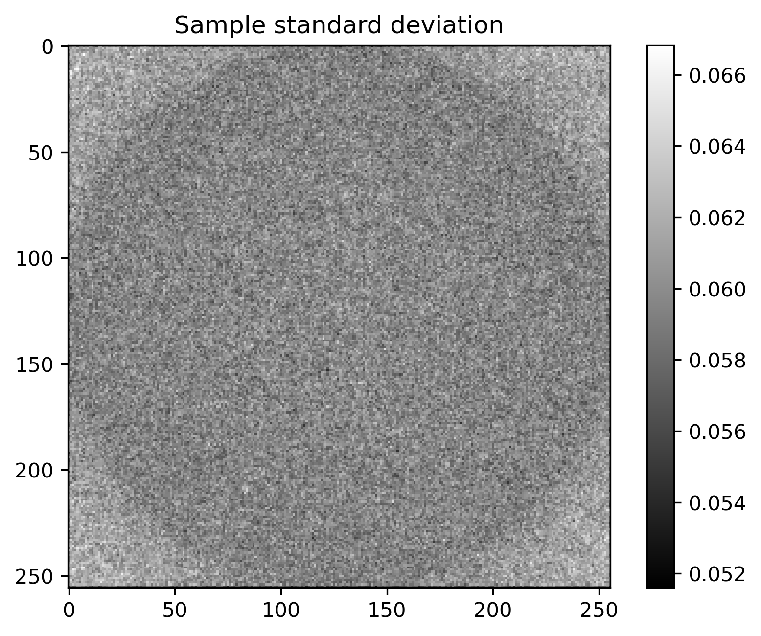
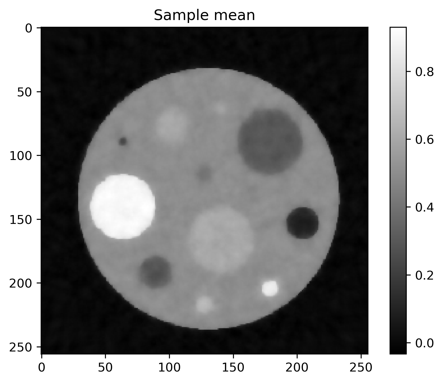
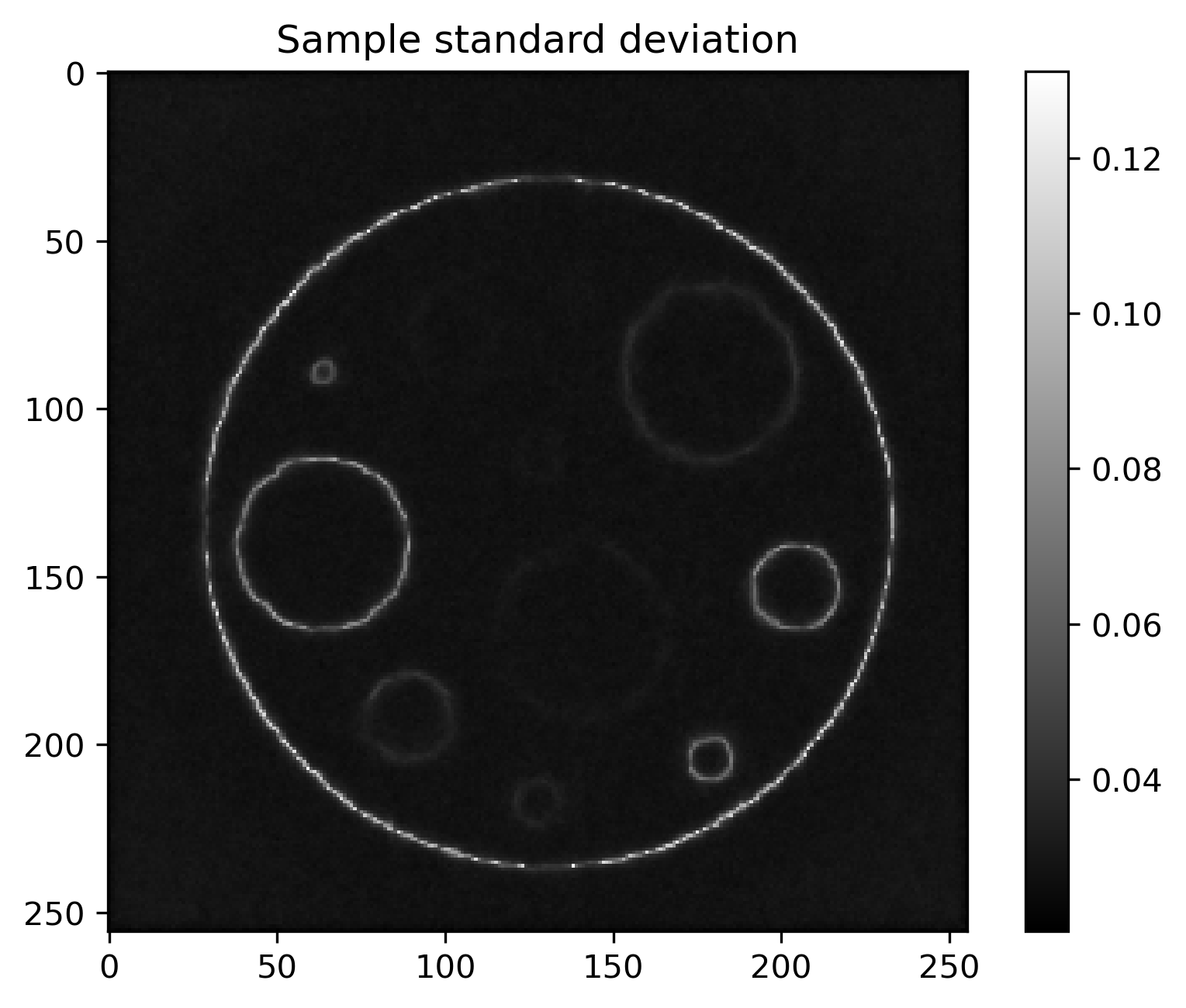
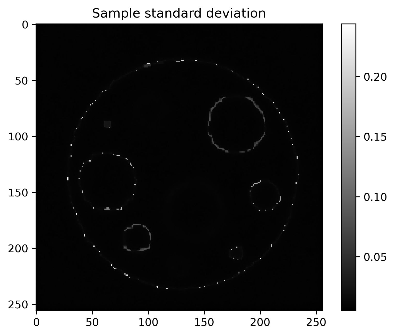
Mean and standard deviation plots for posterior samples using different priors:

Prior	Posterior mean	Posterior std
Gaussian \(\delta=0.01\)
GMRF \(\delta=0.01\)
LMRF \(\delta=0.1\)
CMRF \(\delta=0.01\)

Authors¶

Run¶

docker run -it -p 4243:4243 linusseelinger/benchmark-cuqi-ct

Properties¶

Model	Description
CT_Gaussian	Posterior distribution with Gaussian prior
CT_GMRF	Posterior distribution with Gaussian Markov Random Field prior
CT_LMRF	Posterior distribution with Laplacian Markov Random Field prior
CT_CMRF	Posterior distribution with Cauchy Markov Random Field prior
CT_ExactSolution	Exact solution to the CT problem

CT_Gaussian¶

Mapping	Dimensions	Description
input	[256**2]	Signal \(\mathbf{x}\)
output	[1]	Log PDF \(\pi(\mathbf{b}\mid\mathbf{x})\) of posterior with Gaussian prior

Feature	Supported
Evaluate	True
Gradient	True
ApplyJacobian	False
ApplyHessian	False

Config	Type	Default	Description
delta	double	0.01	The prior parameter \(\delta\) (see below).

CT_GMRF¶

Mapping	Dimensions	Description
input	[256**2]	Signal \(\mathbf{x}\)
output	[1]	Log PDF \(\pi(\mathbf{b}\mid\mathbf{x})\) of posterior with Gaussian Markov Random Field prior

Feature	Supported
Evaluate	True
Gradient	True
ApplyJacobian	False
ApplyHessian	False

Config	Type	Default	Description
delta	double	0.01	The prior parameter \(\delta\) (see below).

CT_LMRF¶

Mapping	Dimensions	Description
input	[256**2]	Signal \(\mathbf{x}\)
output	[1]	Log PDF \(\pi(\mathbf{b}\mid\mathbf{x})\) of posterior Laplacian Markov Random Field prior

Feature	Supported
Evaluate	True
Gradient	False
ApplyJacobian	False
ApplyHessian	False

Config	Type	Default	Description
delta	double	0.01	The prior parameter \(\delta\) (see below).

CT_CMRF¶

Mapping	Dimensions	Description
input	[256**2]	Signal \(\mathbf{x}\)
output	[1]	Log PDF \(\pi(\mathbf{b}\mid\mathbf{x})\) of posterior with Cauchy Markov Random Field prior

Feature	Supported
Evaluate	True
Gradient	True
ApplyJacobian	False
ApplyHessian	False

Config	Type	Default	Description
delta	double	0.01	The prior parameter \(\delta\) (see below).

CT_ExactSolution¶

Mapping	Dimensions	Description
input	[0]	No input to be provided.
output	[256**2]	Returns the exact solution \(\mathbf{x}\) for the deconvolution problem.

Feature	Supported
Evaluate	True
Gradient	False
ApplyJacobian	False
ApplyHessian	False

Config	Type	Default	Description
None

Mount directories¶

Mount directory	Purpose
None

Source code¶

The benchmark is set up in the file server.py as well as data_script.py in the same folder as this readme. The benchmark uses CUQIpy.

Description¶

The CT problem is defined by the inverse problem

\[ \mathbf{b} = \mathbf{A}\mathbf{x} + \mathbf{e}, \]

where \(\mathbf{b}\) is an \(m\)-dimensional random vector representing the observed (vectorized) CT sinogram data, \(\mathbf{A}\) is an \(m\times n\) matrix representing the CT projection operator or “system matrix”, \(\mathbf{x}\) is an \(n\)-dimensional random vector representing the unknown (vectorized) square image, and \(\mathbf{e}\) is an \(m\)-dimensional random vector representing the noise.

The matrix \(\mathbf{A}\) is generated by using the MATLAB package AIR Tools II, described in the publication. Specifically, the following code was used to generate the forward model matrix:

[A, b, x] = paralleltomo(256, 0:6:174, N);
save A256_30.mat A

This corresponds to an image of \(256 \times 256\) pixels, hence \(n=256^2=65536\), scanned in a parallel-beam geometry with 30 projections taking over 180 degrees with angular steps of 6 degrees, each projection consisting of 256 X-ray lines, i.e., \(m = 30*256=7680\). See the above links for more details.

This benchmark defines a posterior distribution over \(\mathbf{x}\) given \(\mathbf{b}\) as

\[ \pi(\mathbf{x}\mid \mathbf{b}) \propto \pi(\mathbf{b}\mid \mathbf{x})\pi(\mathbf{x}), \]

where \(\pi(\mathbf{b}|\mathbf{x})\) is a likelihood function and \(\pi(\mathbf{x})\) is a prior distribution.

The noise is assumed to be Gaussian with a known noise level, and so the likelihood is defined via

\[ \mathbf{b} \mid \mathbf{x} \sim \mathcal{N}(\mathbf{A}\mathbf{x}, \sigma^2\mathbf{I}_m), \]

where \(\mathbf{I}_m\) is the \(m\times m\) identity matrix and \(\sigma=0.01\) defines the noise level.

The prior can be configured by choosing of the following assumptions about \(\mathbf{x}\), where we here consider x a square image with pixels \(x_{i,j}\) for \(i,j = 1, \dots, 256\):

Gaussian: Gaussian (Normal) distribution: \(x_{i,j} \sim \mathcal{N}(0, \delta)\).
GMRF Gaussian Markov Random Field: \(x_{i,j}-x_{i-1,j} \sim \mathcal{N}(0, \delta)\) and \(x_{i,j}-x_{i,j-1} \sim \mathcal{N}(0, \delta)\)
CMRF Cauchy Markov Random Field: \(x_{i,j}-x_{i-1,j} \sim \mathcal{C}(0, \delta)\) and \(x_{i,j}-x_{i,j-1} \sim \mathcal{C}(0, \delta)\)
LMRF Laplace Markov Random Field: \(x_{i,j}-x_{i-1,j} \sim \mathcal{L}(0, \delta)\) and \(x_{i,j}-x_{i,j-1} \sim \mathcal{L}(0, \delta)\)

where \(\mathcal{C}\) is the Cauchy distribution and \(\mathcal{L}\) is the Laplace distribution. The parameter \(\delta\) is the prior parameter and is configurable (see above).

The choice of prior is specified by providing the name to the HTTP model. In this case CT_Gaussian, CT_GMRF, CT_LMRF, and CT_CMRF, respectively. See um-bridge Clients for more details.

In addition to the HTTP models for the posterior, there is also an HTTP model for the exact solution to the problem. This model is called CT_ExactSolution and returns exact phantom used to generate the synthetic data when called.

Using CUQIpy the CT benchmark is defined using the file data_script.py and server.py provided here.