Inferring material properties of a cantilevered beam

Overview

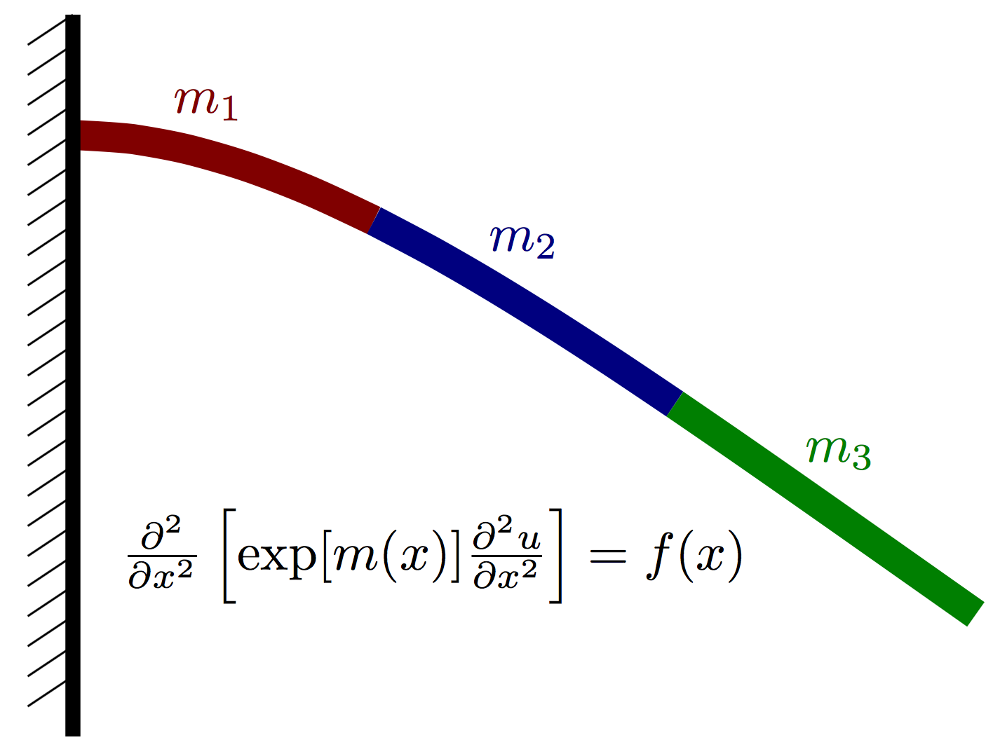
This is a Bayesian inverse problem for characterizing the stiffness in an Euler-Bernoulli beam given observations of the beam displacement with a prescribed load. The Young’s modulus is piecewise constant over three regions. This is shown below.

This docker container uses MUQ and UM-Bridge to evaluate the log posterior density of the problem. Synthetic data is used. A realization of a Gaussian process is used to define a “true” \(m(x)\) that is then run through the PDE model. Additive noise is added to the output of the model to create the synthetic data.

Authors

• Matthew Parno

Run

docker run -it -p 4243:4243 linusseelinger/benchmark-muq-beam:latest

Properties

Model	Description
posterior	Posterior density

posterior

Mapping	Dimensions	Description
input	[3]	The value of the beam stiffness in each lumped region.
output	[1]	The log posterior density.

Feature	Supported
Evaluate	Yes
Gradient	Yes (via finite difference)
ApplyJacobian	Yes (via finite difference)
ApplyHessian	Yes (via finite difference)

Config	Type	Default	Description
None

Mount directories

Mount directory	Purpose
None

Source code

Model sources here.

Description

Let \(u(x)\) denote the vertical deflection of the beam and let \(m(x)\) denote the vertical force acting on the beam at point \(x\) (positive for upwards, negative for downwards). We assume that the displacement can be well approximated using Euler-Bernoulli beam theory and thus satisfies the PDE

\[ \frac{\partial^2}{\partial x^2}\left[ \exp(m(x)) \frac{\partial^2 u}{\partial x^2}\right] = f(x),\]

where \(m(x) = \log E(x)\) is the log of an effective stiffness \(E(x)\) that depends both on the beam geometry and material properties. Our goal is to infer \(m(x)\) given a few point observations of \(u(x)\) and a known load \(f(x)\).

For a beam of length \(L\), the cantilever boundary conditions take the form

\[ u(x=0) = 0,\quad \left.\frac{\partial u}{\partial x}\right|_{x=0} = 0 \]

and

\[ \left.\frac{\partial^2 u}{\partial x^2}\right|_{x=L} = 0, \quad \left.\frac{\partial^3 u}{\partial x^3}\right|_{x=L} = 0. \]

Discretizing this PDE with finite differences (or finite elements, etc…), we obtain a linear system of the form

\[ K(m)\hat{u} = \hat{f},\]

where \(\hat{u}\in\mathbb{R}^N\) and \(\hat{f}\in\mathbb{R}^N\) are vectors containing approximations of \(u(x)\) and \(m(x)\) at finite difference nodes.

We assume that \(m(x)\) is piecwise constant over \(P\) nonoverlapping intervals on \([0,L]\). More precisely,

\[m(x) = \sum_{i=1}^P m_i \,I\left(x\in [a_i, a_{i+1})\right),\]

where \(I(\cdot)\) is an indicator function.

Prior

For the prior, we assume each value is an independent normal random variable

\[m_i \sim N(\mu_i, \sigma_i^2).\]

Likelihood

Let \(N_x\) denote the number of finite difference nodes used to discretize the Euler-Bernoulli PDE above. For this problem, we will have observations of the solution \(u(x)\) at \(N_y\) of the finite difference nodes. Let \(\hat{u}\in\mathbb{R}^{N_x}\) denote a vector containing the finite difference solution and let \(y\in\mathbb{R}^{N_y}\) denote the observable random variable, which is the solution \(u\) at \(N_y\) nodes plus some noise \(\epsilon\), i.e.

\[y = B\hat{u} + \epsilon,\]

where \(\epsilon \sim N(0, \Sigma_y)\). The solution vector \(u\) is given by

\[\hat{u} = [K(m)]^{-1}\hat{f},\]

Combining this with the definition of \(y\), we have the complete forward model

\[y = B[K(m)]^{-1} \hat{f} + \epsilon\]

The likelihood function then takes the form

\[p(y | m) = N\left(\, B [K(m)]^{-1} f,\,\,\Sigma_y \,\right).\]

Posterior

Evaluating the posterior, which is simply written as

\[p(m|y) \propto p(y|m)p(m),\]

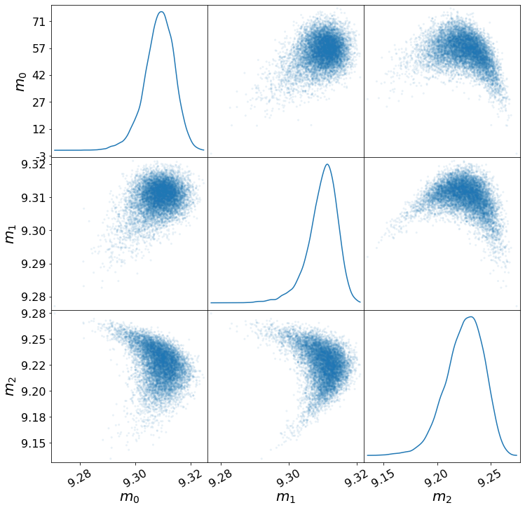
The value of the log posterior density \(\log p(m|y)\) given \([m_1,m_2,m_3]\) is returned by docker container in this benchmark problem.

Samples of the posterior distribution should look like those below.